Easy Deep Learning Part VII

Convolutional Neural Networks #

This is the seventh part of an intended multi-part series on deep learning. You should start with Part 1.

Recap #

By now you should be comfortable with what a neuron is, what a neural network (or a stack of neuron means). We have so far described a neuron to represent g(AX + b) which was chained together in multiple layers that created a deep network. Next we talked about concepts like dropout, different activation function, regularization and different initialization to get better results.

What is missing? #

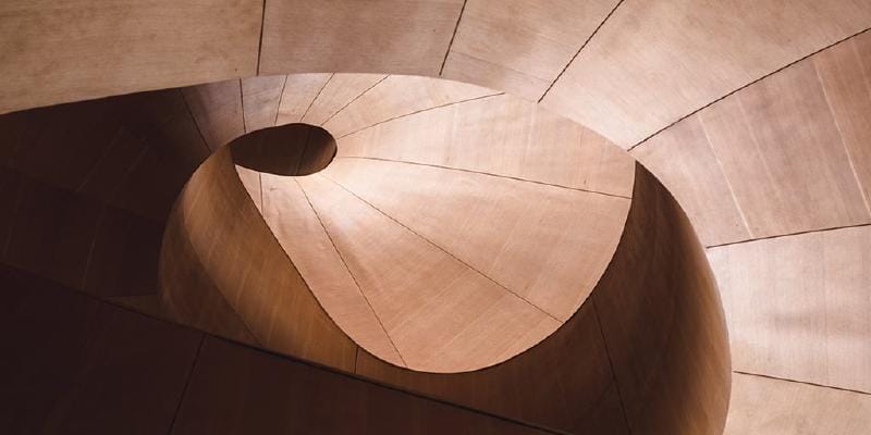
When I described the core concept of having depth, I talked about teams looking at different parts of the image adn giving a decision. But when we implemented it, we created a dense layer where everyone looks at everything. And we know that that may be a bad use of resources. Most information in the image is associated close to each other. Randomly arranging the eyes, nose and ears won’t make a face and looking at random places for that is definitely not a great idea. Therefore it makes sense to have teams look at small parts and then take their decision. The next question would be team size. The bigger the teams, the closer we get to the original dense network problem. Therefore its better to start with the smallest teams and look grow them if things don’t work well. So what is the smallest team size. An image is two dimensional(actually 3 because of RGB, but since the third dimension is so small, we don’t really talk about that in our convolutions here) and therefore, we need a 2D convolution. The smallest symmetrical one is everyone looking at one pixel. But then we can’t build a hierarchy with one element in the next layer looking at only 1 pixel(1x1) (There is a 1x1 module you might find in certain networks. It is too advanced for now. We discuss that in part 10.). What is the next one. It is not 2x2. Because we cannot chose which 2 we need(left or right). Therefore it has to be 3x3 i.e. 9 pixels. People have tried 5 and 7 pixel rows but have realized over time that adding another layer is better than making it bigger. It is faster because of lesser variables and leaves little reason to go higher (More on this in Post 10). So how does it look like to a user. You can get a fair idea from the visualization from vdumoulin displayed in the first image below.

Ideas from classical computer vision #

Convolutions are not a new concept. They have been there in computer vision for a long time. The idea of a convolution is very simple. If you look at an image, one thing you definitely see is the color, but color in itself is not very interesting. It is the change in color that interests us. The change in color across individual pixels is is really what defines everything. Smooth change would probably mean a gradient, zero change would be solid color and a huge change would be an edge. A lot of effort has already gone into finding hand coded kernels (specific values of these convolutions) for detection of edges corners etc. as well as for styling images into different variants like blurring or sharpening.

You can play with and understand the concepts using the visualization here.

Size problems #

You might have noticed, the approach above would reduce the output prediction size by two pixels in both rows and columns. Going back to manager analogy, each manager has 9 people reporting, but not all people have 9 managers. The pixels at the edges don’t have all neighbors and therefore the calls from the higher level don’t really center them. In a classic organization that is not a problem (rather a good thing). You may assume that since we want a single number as an output, it is a good thing. And I would agree. But there is one reason why we want this to be the same. The reason is simple. We want to stack multiple layers. We cannot go very deep if we reduce pixels each time. Also we will have to write separate layers for each kernel size. We cannot try different model pieces at different parts of the network and all that together makes our work difficult. Therefore we add padding to the original image so that it becomes consistent. The padding is all zeros and a smart network should be able to set the scores properly that those pixels won’t matter. Anyways, if x is 0, ax is also gonna be 0. The second image below is another image from the same visualization on padding.

More tricks #

Stride: You might have also noticed that reporting to 9 managers is sort of a confusing. There is a lot of duplication of information. Of course it is good to some extent that the same pixel can be measured differently, but do remember that the basic thing we did with MNIST worked well. There might not be enough information in a single signal(pixel or manager’s output), to require a huge set of weights looking at it. Therefore to speed up the network we use a stride, i.e. have only a few center pixels and consolidate the output. You can understand stride by the third visualization easily. Transpose With a stride we lose the benefits we added padding for. So we add the padding back to get to the same size via a transpose. The fourth visualization explains this concept.

Maxout/Averageout #

There is one more concept that needs to be understood before going to code. This one is more of an optimization than a real trick. We can run multiple convolutions on the input data and it is a good idea to do that. This is because one convolution ideally carries only type of information. Eg one convolution could be a line detector, a corner detector, a blob or circle detector etc. With many convolutions on a big image we have a lot of data. We reduce this for getting better performance. There are many ways to reduce data, averaging(Averageout), picking up up one of them or picking up a min or max. Maxout or picking up the max in a set is very popular. We run a convolution and pick up the max of a small kernel (convolution area like 9 pixels) and keep that discarding the others. Why Max- because based on the intuitions from ReLU it seems like a good idea. But we are free to try other optimizations. It is an important trick to summarize the inputs and that is why very popular especially after a few Conv layers.

Convolutions outside images #

The concepts of dividing local stuff and then putting a manager onto global stuff is not just applicable to images. Words are formed by looking at nearby characters, sentences via words and paragraphs via sentences. So this logic can be used on sentences of text. This logic can also be used with voice as that also consists of a similar pattern. I hope you can imagine how these simple concepts change everything.

Summary #

Here we discussed the intuition and some concepts around Convolutions and why having local information passed onto the next layer is a good idea.

In the next post we will apply this to the CIFAR data set and show some results from the convolutional neural networks that can really amaze us all.