
Easy Deep Learning Part IV
Working code #
This is the fourth part of an intended multi-part series on deep learning. You should start with Part 1.
Recap #
In the previous sections we defined our deep learning task of identifying the contents of an image:
g(AX + b) = Probability of being a content type
where X is the huge matrix that makes up the image and A are the weights, b the biases and g is the function that converts scores into probabilities like softmax.
We realized that the traditional way of solving equations does not work well with this case and therefore we described SGD as a means to solve the equation to get A and b.
Technical Considerations #
I hope you feel the same as me right now that deep learning as a concept is not very difficult. We use a very simple equation, fill it up with random numbers and slowly tweak that until we are done. The challenge comes up with the implementation. In any practical use case we are talking about a few million multiplications per image. Now that means we need a beefy GPU as running those multiplications one by one will turn out to be very slow. Add to that, we need floating point numbers (not integers) which take more space (4 bytes by default). Therefore for a single 1 megapixel image we are talking about 3GB of GPU memory to store A alone. Still it takes hours to train. The ImageNet model that is used to recognize images takes a month on a cluster of 5 of the fastest GPU available.
So make some compromises:
- We take small images and most of the time their size is a power of 2.
- We train in batches. Since gradient calculation is very expensive, we run the forward pass for multiple images at a time and once one set of images goes through we calculate the overall loss across all those images and push that back into the equation.
- Deep learning libraries do most of the heavy lifting for us and automatically divide between the various machines, effectively use the GPU, and also calculate the gradient to run the back propagation. We just define the model.
- Because of the very specific input requirements, the data gathering is the toughest part of a deep learning system. We need to clean the data and get it to the correct shape and sizes.
Libraries #
This is a very biased topic. I don’t want to go in the benefits and disadvantages of a library. Any ways, if you are not doing research but instead just tweaking something that is already there(which you should be doing), there is no point in arguing about it. All are good enough. The biggest guns in the market are with caffe (facebook), tensorflow(google) and CNTK(microsoft). Again the goals of all these libraries are different. They are made for modifying the core of the networks, and messing up with the stuff like calculus which you don’t need to go into just right now.
For the sake of simplicity, I use keras. This is one of the simplest to use libraries with the minimal amount of code you need to write. The library is built over CNTK, tensorflow and theano and therefore you can go deep into lower level if you so desire. This library also enables me to export models that you can visualize in Javascript. Since it is built over tensorflow, you can export its models to mobile and run them there.
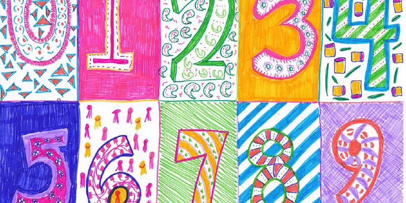
MNIST #
The MNIST data set is a data set of black and white (saves us the RGB channels) images of handwritten numbers(not cat pictures) from 0-9 all labelled correctly. They are available as 28x28 pixel images (not 1 megapixel). It is a very popular data set for trying out complicated networks as the problem is just perfect - not too heavy to require huge amount of processing time, not simple to be solvable easily by other means and not too complicated so that it can be solved by the simplest of neural networks.
Installation #
From the python website install python. Remember to enable pip(or use get-pip.py to download pip). Then run pip install keras to get keras.
You can now run python files by python filename. Google is your friend here (better than me) and you can always go to keras.io to find the latest installation instructions.
Code #
- Import the python modules to use
| |
- Load the data Now keras comes bundles with MNIST. This is a data set of handwritten numbers (0-9). The images are all 28x28 and labelled with the correct number. Keras defines 60k images in the training and 10k in the testing set.
| |
- Fit the data to our equation We do not use the fact that the image is 2 dimensional. we just create a flat list of 784 numbers. The -1 in the reshape is to keep the first dimension with the remaining dimension. We create 1 matrix of size [1x784] for each image and put all the images one under the other. Also the output is written as a single number. We convert that to categories, i.e. 1 row per output. This is because we want the probabilities of each number (0, 1, 2..9) separately. This type of encoding is called categorical or one hot encoding. In a more advanced network, we can also keep this as a single number where the equation outputs between 0 & 0.1 for 1, 0.1 & 0.2 for 2 and so on. Probabilities are easier to understand and therefore we like the one hot output.
| |
- Define our equation The equation is called a model in keras. The code is should be very intuitive. You can ignore the term Sequential for now, since we have only one element, that does not technically mean a sequence. Next is Dense with 10 outputs and 784 inputs. Here we define the size of
y&XinAX + b = y. The size ofAandbis inferred by the network automatically. Dense means all inputs and outputs are connected. We will get into other types of networks later. The activation function is softmax, the only one we have discussed so far.
| |
- Define the loss function We apply cross entropy loss to multiple categories. The optimization algorithm is SGD and we are looking for better accuracy.
| |
- Run the training set This method takes a lot of time. This takes the batch size(to group multiple images in a single pass) and the number of epochs(number of times to run this).
| |
That is it. We have a trained model. Now we can pass a new image and get the corresponding probabilities. To verify the accuracy of our model (remember the over fitting problem. We need to know how it performs in a new unseen data set) use test the model
| |
This should give you an accuracy of 92-93%. Just like that.
Here is the full code:
| |
Now that we have working code, we can really zoom ahead. You know the basics. Give me some time to build upon it. In part 5 we will talked about deeper networks, how and why.
Comments
Post a new comment
We get avatars from Gravatar. You can use emojis as per the Emoji cheat sheet.